Differential Geometry
Differential geometry at its most fundamental is the study of curves and surfaces in three-dimensional space. It is then generalised to higher dimensions including surfaces that are not necessarily Euclidean (flat) that Riemannian geometry focuses on, i.e. on Riemannian manifolds.
To start off, we will explore various fundamental concepts and tools in Euclidean space, particularly surfaces in \( \mathbb{R}^3 \).
Length of Curves, Volume of Surfaces and the First Fundamental Form
Maximisation, Minimisation and the Second Fundamental Form
In this section, we will consider the concepts of maximisation and minimisation of functions defined on surfaces, as well as the second fundamental form which encodes information about the curvature of a surface. We will first consider a function \( f: \mathbb{R}^n \to \mathbb{R} \). It can be particularly helpful to think of the function as a surface lying in \( \mathbb{R}^3 \) first (where \( n=2 \)) and generalise to higher dimensions. To find the maximum or minimum of the function, one should think of the tangent plane across the surface at some point \( p \). The tangent plane is simply a generalisation of the tangent line to curves in \( \mathbb{R}^2 \) where you can construct it by considering all paths \( \gamma: (-\epsilon, \epsilon) \to f(\mathbb{R}^2) \) such that \( \gamma(0) = p \) and taking the span of all tangent vectors \( \gamma'(0) \). Simply put, the tangent plane tells you in which direction on the surface the function will go and if it is completely flat, then that means that the function either will not move up or down and therefore you have a maxima or minima locally. There is also another case of it being a saddle point which is reflective of the inflection point of functions on the Cartesian plane
— in this case, the function looks flat at the point but it increases and decreases in different directions like a saddle.
Therefore, to find the points where the function has a maxima or minima, we need to find when
$$ \nabla f = 0 $$ which represents when all the partials are 0, because the partials represent the slope of the function in each direction and the slope at any direction is a linear combination of the partials. We will now derive the Taylor expansion of the function at a point \( p \) to second order to see how the function behaves around that point. Consider \( g(h) = f(x+hv) \) where \( v \) is some direction vector and \( h \) is a scalar. Then by Taylor's theorem for one-dimensional Taylor series, we have
$$ g(h) = g(0) + g'(0)h + \frac{g''(0)}{2}h^2 + O(h^3) $$
where \( O(h^3) \) represents the higher order terms. Now, by the multivariate chain rule, we have
\begin{align*}
g'(h) &= \nabla f(x+hv) \cdot v \\
\implies g'(0) &= \nabla f(x) \cdot v
\end{align*}
and similarly, we can differentiate again to get
\begin{align*}
g''(h) &= \frac{d}{dh}\sum_{i=1}^n \frac{\partial f}{\partial x_i}(x+hv) v_i \\
&= \sum_{i=1}^n \sum_{j=1}^n \frac{\partial^2 f}{\partial x_i \partial x_j}(x+hv) v_i v_j \\
&= v^T H_f(x+hv) v
\implies g''(0) = v^T H_f(x) v
\end{align*}
where \( H_f \) is the Hessian matrix of \( f \) given by
$$ H_f = \begin{bmatrix}
\frac{\partial^2 f}{\partial x_1^2} & \frac{\partial^2 f}{\partial x_1 \partial x_2} & \cdots & \frac{\partial^2 f}{\partial x_1 \partial x_n} \\
\frac{\partial^2 f}{\partial x_2 \partial x_1} & \frac{\partial^2 f}{\partial x_2^2} & \cdots & \frac{\partial^2 f}{\partial x_2 \partial x_n} \\
\vdots & \vdots & \ddots & \vdots \\
\frac{\partial^2 f}{\partial x_n \partial x_1} & \frac{\partial^2 f}{\partial x_n \partial x_2} & \cdots & \frac{\partial^2 f}{\partial x_n^2}.
\end{bmatrix} $$
Therefore, substituting back into the Taylor expansion, we have
$$ f(x+hv) = f(x) + \nabla f(x) \cdot v h + \frac{1}{2} v^T H_f(x) v h^2 + O(h^3) $$
or more generally, for some vector \( v \) close to 0, we have
$$ f(x+v) = f(x) + \nabla f(x) \cdot v + \frac{1}{2} v^T H_f(x) v + O(\|v\|^3). $$ At the critical points, we have
$$ f(x+v) = f(x) + \frac{1}{2} v^T H_f(x) v + O(\|v\|^3). $$
We will now show that the definiteness of the Hessian matrix \( H_f(x) \) determines the nature of the critical point, making use of the fact that the \( O(\|v\|^3) \) term becomes negligible as \( v \) approaches 0. To do this, we consider the Rayleigh quotient
$$ R(v) = \frac{v^T H_f(x) v}{\|v\|^2}. $$
As \( H_f(x) \) is symmetric (when second partials are continuous by Schwarz' Theorem), we can diagonalise it with respect to an orthonormal basis. Let the eigenvalues and corresponding eigenvectors be \( \lambda_1, \ldots, \lambda_n \) and \( e_1, \ldots, e_n \), respectively. Then we can write any vector \( v \) as
$$ v = \sum_{i=1}^n c_i e_i. $$ Let \( \alpha = \min_{1 \leq i \leq n} \lambda_i \) and \( \beta = \max_{1 \leq i \leq n} \lambda_i \).
Now, from the Rayleigh quotient, we have
\begin{align*}
R(v) &= \frac{v^T H_f(x) \left( \sum_{j=1}^n c_j e_j \right)}{\| v\|^2} \\
&= \frac{v^T \sum_{j=1}^n c_j H_f(x) e_j}{\| v\|^2} \\
&= \frac{v^T \sum_{j=1}^n c_j \lambda_j e_j}{\| v\|^2} \\
\implies R(v) &\leq \beta \frac{v^T \sum_{j=1}^n c_j e_j}{\| v\|^2} = \beta \\
\text{and } R(v) &\geq \alpha \frac{v^T \sum_{j=1}^n c_j e_j}{\| v\|^2} = \alpha. \\
\end{align*}
Therefore, $$ \alpha \leq R(v) \leq \beta$$ and for all \( v \neq 0 \) near 0, we have
\begin{align*}
f(x+v) - f(x) &= \|v\|^2 \left ( \frac{1}{2} \frac{v^T H_f(x) v}{\|v\|^2} + O(\|v\|) \right ) \\
&= \|v\|^2 \left ( \frac{1}{2} R(v) + O(\|v\|) \right ).
\end{align*}
For large enough \( v \), the \( O(\|v\|) \) term can be made arbitrarily small. Therefore, we have the following cases:
- If \( H_f(x) \) is positive definite (i.e. all eigenvalues are positive), then \( \alpha > 0 \) and thus \( f(x+v) - f(x) > 0 \) for all \( v \neq 0 \) near 0, indicating a local minimum at \( x \).
- If \( H_f(x) \) is negative definite (i.e. all eigenvalues are negative), then \( \beta < 0 \) and thus \( f(x+v) - f(x) < 0 \) for all \( v \neq 0 \) near 0, indicating a local maximum at \( x \).
- If \( H_f(x) \) is indefinite (i.e. has both positive and negative eigenvalues), then there exist directions \( v_1 \) and \( v_2 \) such that \( f(x+v_1) - f(x) > 0 \) and \( f(x+v_2) - f(x) < 0 \), indicating a saddle point at \( x \).
We now look at curvature. It is analogous to the second derivative of functions in one dimension. Similar to how we looked at each direction on the surface to find the tangents, we look at the curvature in each direction on the surface. Once again, we consider
$$ \frac{d^2}{dt^2} f(x + tv) \bigg|_{t=0} = v^T H_f(x) v. $$ By using the same eigenvalues and eigenvectors as above, we can rewrite \( v \) as
$$ v = \sum_{i=1}^n c_i e_i. $$ Then, we have
\begin{align*}
v^T H_f(x) v &= \left( \sum_{i=1}^n c_i e_i \right)^T H_f(x) \left( \sum_{j=1}^n c_j e_j \right) \\
&= \sum_{i=1}^n \sum_{j=1}^n c_i c_j e_i^T H_f(x) e_j \\
&= \sum_{i=1}^n \sum_{j=1}^n c_i c_j \lambda_j e_i^T e_j \\
&= \sum_{i=1}^n c_i^2 \lambda_i,
\end{align*}
by orthogonality of the eigenvectors. Therefore, the curvature in the direction of an eigenvector \( e_k \) is the corresponding eigenvalue \( \lambda_k \). A positive eigenvalue indicates that the surface curves upwards in that direction and a negative eigenvalue indicates that the surface curves downwards. If all eigenvalues are positive, the surface is locally convex and if all eigenvalues are negative, the surface is concave. We call the eigenvalues the principal curvatures of the surface at point \( p \). Note that \( \alpha \sum_{i=1}^n c_i^2 \leq \sum_{i=1}^n c_i^2 \lambda_i \leq \beta \sum_{i=1}^n c_i^2 \) so that curvature is bounded by the principal curvatures.
Denote the principal curvatures by \( \kappa_i \) and let \( n=2 \) for surfaces in \( \mathbb{R}^3 \). Then, we have the following curvatures
- \( H = \frac{\kappa_1 + \kappa_2}{2} \) which is the mean curvature and
- \( K = \kappa_1 \kappa_2 \) which is the Gaussian curvature.
Specifically, if \( K > 0 \), the surface is locally shaped like a sphere (elliptic point). If \( K < 0 \), the surface is locally shaped like a saddle (hyperbolic point) and if \( K = 0 \), the surface is locally shaped like a cylinder (parabolic point). The surface is locally called an
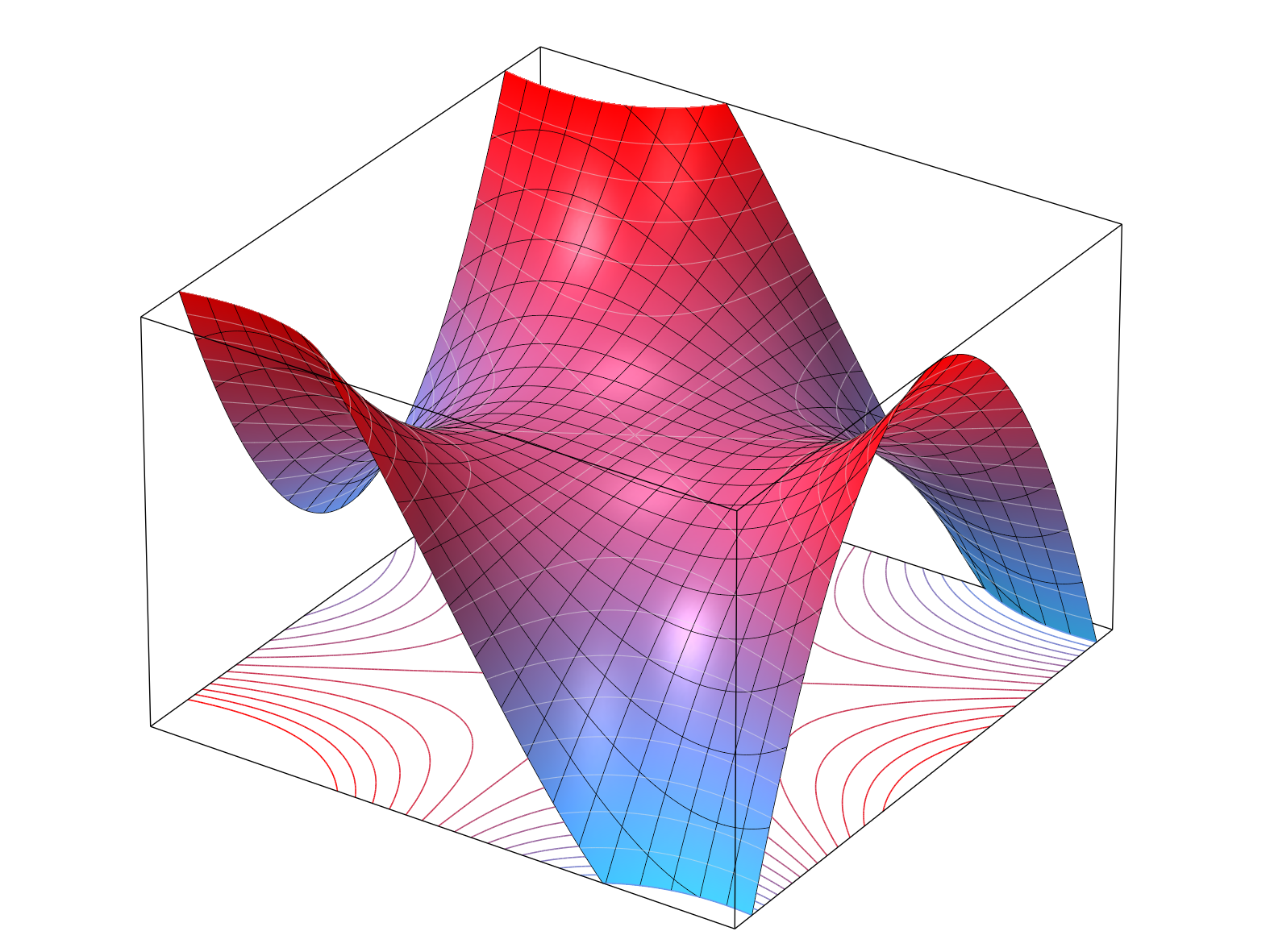
umbilic point if the curvatures are the same in all direction (so it curves the same in all directions). A special case is the flat umbilic point where the curvatures are uniformly 0 so the surface locally looks like a plane — one such example is the
monkey saddle.
The Second Fundamental Form in our special case is defined as the Hessian which encodes all the curvature information of the surface at a point. It is denoted by \( II_p \) at point \( p \). We will later generalise this onto Riemannian manifolds.